Expressions

Through out Verilog-A/MS mathematical expressions are used to specify behavior. Expressions are made up of operators and functions that operate on signals, variables and literals (numerical and string constants) and resolve to a value. Operators and functions are describe here. Signals, variables and literals are introduced briefly here and described in more depth in their own sections (Numbers, signals and Variables).

Literals

Literals are values that are specified explicitly. Their values are fixed; they cannot change. For this reason, literals are often referred to as constants, but it is important that recognize that constants is a term that encompasses other things besides literals. For example, parameters are constants but are not literals.

The following are examples of literals:

0, 27, 8'b1001_1100
are all integer literals,
0.0, 2.2p and 8.8e-12
are all real literals, and
"hello world.\n"
is a string literal.

Variables

Variables are names that refer to a stored value that can be changed. To access the value of a variable, simply use the name of the variable in an expression.

You can access individual members of an array by specifying the desired element as an index. For example:

coefs[3]

accesses element 3 of coefs. You can create a sub-array by using a range or an integer array as an index. For example:

coefs[3:0]
coefs[{5,3,1}]

You cannot directly use an array in an expression except as an index.

Similarly, all three forms of indexing can be applied to integer variables.

Signals

Signals are the values on structural elements used to interconnect blocks in a design, including wires, nets, ports, and nodes. There are two basic kinds of signals: continuous and discrete. With discrete signals the values change only at discrete points in time, meaning that they are piecewise constant. There are two kinds of discrete signals, those with binary values and those with real values. Continuous signals can vary continuously with time. Continuous signals are always real. In addition, signals can be either scalars or vectors. A vector signal is referred to as a bus.

Discrete Signals

One accesses the value of a discrete signal simply by using the name of the wire, net, or port that carries the signal in an expression.

If the signal is a bus of binary signals then by using the its name in an expression you will get all of the members of the bus interpreted as either an unsigned binary number or a 2’s complement number. For example, if gain is a 4-bit unsigned port and if the value of its 4-bits are 1,1,1,1, then when used in an expression it will be interpreted as the value 15.

You can access an individual member of a bus by appending [i] to the name of the signal, where i is index of the member you desire (ex. gain[0]). To access a range of members, use [i:j] (ex. gain[2:0]). To access several possibly non-adjacent members, use [{i,j,k}] (ex. ctrls[{12,5,4}]).

Continuous Signals

With continuous signals there are always two components associated with the underlying structural element (node or port). For example, with electrical signals the two components are the voltage and the current. Thus to access a continuous signal it is not sufficient to simply give of the name of the node or port that carries the signal, you must embed that name within an access function that is used to access the component you want. With electrical signals, there are two access functions: V and I. The first accesses the voltage and the second accesses the current. So, if you would like the voltage on the vdd port, you would use V(vdd).

Continuous signals also can be arranged in buses, and since the signals have real values, a bus of continuous signals cannot be used directly in an expression. It is necessary to pick out individual members of the bus when using the bus in an expression. In this case, the index must be a constant or a genvar. For example, an output behavior of a port can be described as:

v = 5 * V(in[1])

In this case, the output voltage will be the voltage of the in[1] port multiplied by 5.

Operators

Operators are applied to values in the form of literals, variables, signals and expressions to produce new values. One or more operator applied to one or more values is referred to as an expression. Thus you can use an operator on an expression to build another expression, and by doing so you can build up expressions of arbitrary complexity.

No operations are allowed on strings except concatenate and replicate.

Verilog-A/MS supports the operators described in the following tables:

Arithmetic Operators

Symbol	Usage	Description
`+`	`a + b`	Sum `a` and `b`
`+`	`+a`	`a`
`-`	`a - b`	Subtract `b` from `a`
`-`	`-a`	Negate `a`
`*`	`a * b`	Multiply `a` and `b`
`/`	`a / b`	Divide `a` by `b`
`%`	`a % b`	Modulus (remainder) of `a/b`
`**`	`a ** b`	`a` raised to the power of `b`

The result of 5 + 2 is 7.
The result of 5 - 2 is 3.
The result of -5 - 2 is -7.
The result of 5 * 2 is 10.
The result of 5 / 2 is 2.
The result of 5 % 2 is 1.
The result of -5 % 2 is -1 (takes sign of first operand).
The result of 5 % -2 is 1 (takes sign of first operand).
The result of 5 ** 2 is 25.

If either operand of an arithmetic operator is real, the other is converted to real before performing the operation. If both operands are integers, the result will be an integer (rounded towards 0).

The result of 1 / 2 is 0.
The result of 1.0 / 2 is 0.5.
The result of 1 / 2.0 is 0.5.
The result of 1.0 / 2.0 is 0.5.

The result of 1.0 * 4'bF is 15.0.

When the operands are sized, the size of the result will equal the size of the operand with the largest size. Simple integers are 32 bit numbers.

The result of 1'b0 & 3'o7 is 3'o7.
The result of 1'b1 & 3'o7 is 3'o0.
The result of 4'hF + 1 `` is ``32'h10.

If both operands are integers and either operand is unsigned, the result is unsigned. Simple integers are signed numbers.

The result of 8'h00 - 8'01 is 8'hFF.

The result of 8'h00 - 1 is 32'h100000000 or 4294967296.

Bitwise Operators

Symbol	Usage	Description
`~`	`~a`	Invert each bit of `a`
`&`	`a&b`	Logical ‘and’ of each bit of `a` and `b`
`~&`	`a~&b`	Logical ‘nand’ of each bit of `a` and `b`
`\|`	`a\|b`	Logical ‘or’ of each bit of `a` and `b`
`~\|`	`a~\|b`	Logical ‘nor’ of each bit of `a` and `b`
`^`	`a^b`	Logical ‘xor’ of each bit of `a` and `b`
`~^`	`a~^b`	Logical ‘xnor’ of each bit of `a` and `b`
`^~`	`a^~b`	Same as `~^`

The result of ~ 'b1011 is 'b0100.
The result of 'b1001 & 'b1010 is 'b1000.
The result of 'b1001 ~& 'b1010 is 'b0111.
The result of 'b1001 | 'b1010 is 'b1011.
The result of 'b1001 ~| 'b1010 is 'b0100.
The result of 'b1001 ^ 'b1010 is 'b0110.
The result of 'b1001 ~^ 'b1010 is 'b1001.
The result of 'b1001 ^~ 'b1010 is 'b1001.

The operator first makes both the operand the same size by adding zeros in the most-significant bit positions in the operand with the smaller size. It then computes the result by performing the operation bit-wise, meaning that the operation is performed for each pair of corresponding bits, one from each operand.

The result of 'b00 & 'b11 is 'b00.
The result of 'b01 & 'b11 is 'b01.
The result of 'b10 & 'b11 is 'b10.
The result of 'b11 & 'b11 is 'b11.

The bitwise operators cannot be applied to real numbers.

Reduction Operators

Symbol	Usage	Description
`&`	`&a`	Logical ‘and’ all bits in `a` to form 1 bit result
`~&`	`~&a`	Logical ‘nand’ all bits in `a` to form 1 bit result
`\|`	`\|a`	Logical ‘or’ all bits in `a` to form 1 bit result
`~\|`	`~\|a`	Logical ‘nor’ all bits in `a` to form 1 bit result
`^`	`^a`	Logical ‘xor’ all bits in `a` to form 1 bit result
`~^`	`~^a`	Logical ‘xnor’ all bits in `a` to form 1 bit result
`^~`	`^~a`	Same as `~^`

The reduction operators start by performing the operation on the first two bits of the operand, it then performs the operation on the result and the third bit. This process is continued until all bits are consumed, with the result having only 1 bit.

The result of &'b1010 is 1'b0.
The result of ~&'b1010 is 1'1.
The result of |'b1010 is 1'b1.
The result of ~|'b1010 is 1'b0.
The result of ^'b1010 is 1'b1.
The result of ~^'b1010 is 1'b0.
The result of ^~'b1010 is 1'b0.

The reduction operators cannot be applied to real numbers.

Logical Operators

Symbol	Usage	Description
`!`	`!a`	Is `a` false?
`&&`	`a&&b`	Are both `a` and `b` true?
`\|\|`	`a\|\|b`	Are either `a` or `b` true?

The logical operators take an operand to be true if it is nonzero. They return a one bit result of 1 if the result of the operation is true and 0 otherwise.

The result of !0 is 1.
The result of !1 is 0.
The result of !2 is 0.
The result of !'hF is 0.
The result of !'bX is 1'bX.
The result of 73 && 17 is 1.
The result of 73 && 'bX is 1'bX.
The result of -73 || -17 is 1.
The result of -73 || 'bX is 1'bX.

Equality Operators

Symbol	Usage	Description
`==`	`a==b`	Is `a` equal to `b`?
`!=`	`a!=b`	Is `a` not equal to `b`?

The equality operators evaluate to a one bit result of 1 if the result of the operation is true, 0 if the result is false, and x otherwise. Thus, if either operand contains an x the result will be x.

The result of 0 == 0 is 1.
The result of 1 == 0 is 0.
The result of 'bX == 0 is 'bX.
The result of 'bZ != 0 is 'bX.

Identity Operators

Symbol	Usage	Description
`===`	`a===b`	Is `a` identical to `b`?
`!==`	`a!==b`	Is `a` not identical to `b`?

The identity operators evaluate to a one bit result of 1 if the result of the operation is true, 0 if the result is false. The result of the operation is either true or false, so the identity operators never evaluate to x.

The result of 0 === 0 is 1.
The result of 1 === 0 is 0.
The result of 'bX === 0 is 0.
The result of 'bZ === 0 is 0.
The result of 'bX === 'bX is 1.
The result of 'bZ !== 'bX is 1.

Relational Operators

Symbol	Usage	Description
`<`	`a<b`	Is `a` less than `b`?
`>`	`a>b`	Is `a` greater than `b`?
`<=`	`a<=b`	Is `a` less than or equal to `b`?
`>=`	`a>=b`	Is `a` greater than or equal to `b`?

The relational operators evaluate to a one bit result of 1 if the result of the operation is true, 0 if the result is false, and x otherwise. Thus, if either operand contains an x or z the result will be x.

The result of 73 < 73 is 0.
The result of 73 > 73 is 0.
The result of 73 <= 73 is 1.
The result of 73 >= 73 is 1.
The result of 73 < 'bX is 'bX.
The result of 73 >= 'bX is 'bX.

Shift Operators

Symbol	Usage	Description
`<<`	`a<<b`	Shift `a` left `b` bits, vacated bits are filled with 0
`>>`	`a>>b`	Shift `a` right `b` bits, vacated bits are filled with 0
`<<<`	`a<<<b`	Shift `a` left `b` bits, vacated bits are filled with 0
`>>>`	`a>>>b`	Shift `a` right `b` bits, vacated bits are filled with 0 if `a` is unsigned and by the sign bit of `a` otherwise

The right operand is always treated as an unsigned number and has no affect on the signedness of the result. If the right operand contains an x, the result is x.

The result of 4'b0011 << 0 is `4'b0011.
The result of 4'b0011 << 1 is `4'b0110.
The result of 4'b0011 << 2 is `4'b1100.
The result of 4'b0011 << 3 is `4'b1000.
The result of 4'b0011 << 4 is `4'b0000.
The result of 4'b0011 >> 1 is `4'b0001.
The result of 4'b10011 >> 1 is `4'b01001.

Arithmetic shift operators fill vacated bits on the left with the sign bit if expression is signed, otherwise it fills with zero.

The result of 4'b0011 >>> 1 is `4'b0001.
The result of 4'sb0011 >>> 1 is `4'sb0001.
The result of 4'b1111 >>> 1 is `4'b0111.
The result of 4'sb1111 >>> 1 is `4'sb1111.
The result of 4'b0011 <<< 1 is `4'b0110.
The result of 4'b1111 <<< 1 is `4'b1110.
The result of 4'sb0011 <<< 1 is `4'b0110.
The result of 4'sb1111 <<< 1 is `4'b1110.

The left arithmetic shift (<<<) is identical to the left logical shift (<<).

The shift operators cannot be applied to real numbers.

Miscellaneous Operators

Symbol	Usage	Description
`?:`	`a ? b : c`	Evaluated to `b` if `a` is true and `c` otherwise
`{}`	`{a,b}`	Concatenates sized bit vectors `a` and `b`
`{{}}`	`{a{b}}`	Replicate `b`, `a` times

The result of 0 ? 73 : 17 is 17.
The result of 1 ? 73 : 17 is 73.
The result of 'bX ? 73 : 17 is 17.
The result of {4'b1100, 2'b11} is 6'b110011.
The result of {4{2'b01} is 8'b0101010101.

The concatenation and replication operators cannot be applied to real numbers.

Sign and Size of Result

When an operator produces an integer result, its size depends on the size of the operands. The following table gives the size of the result as a function of the operator and form where L(i) represents the size (length) of argument i:

Form	Operators	Size
i op j	`+`, `-`, `*`, `/`, `%`, `&`, `\|`, `^`, `^~`	max(L(i), L(j))
op i	`+`, `-`, `~`	L(i)
i op j	`==`, `!=`, `===`, `!==`, `&&`, `\|\|`, `>`, `>=`, `<`, `<=`	1
op i	`&`, `~&`, `\|`, `~\|`, `^`, `~^`	1
i op j	`>>`, `<<`	L(i)
i ? j : k		max(L(j), L(k)
{i, …, j}		L(i) + … + L(j)
{i {j, …, k}}		i `*` (L(j) + … + L(k))

When an operator is applied to an unsigned integer, the result is unsigned. When a binary operator is applied to two integer operands, one of which is unsigned, the result is generally unsigned.

For those that are used to only working with reals and simple integers, use of sized and unsigned integers can cause very unexpected results. For example, if you add two 4-bit numbers the result will be 4-bits, and so any carry would be lost. For example, the result of 4’d15 + 4’d15 is 4’d14. This odd result occurs because there is only 4-bits available to hold the result, so the most significant bit is lost (Verilog is a hardware description language, and this is the way a 4-bit adder without carry would work). Similar problems can arise from the unsigned nature of these integers. For example, 8’h00 - 1 is 4,294,967,295. To see why, take it one step at a time.

8’h00 is an 8-bit unsigned number.
1 is an unsized signed number. Unsized numbers are represented using 32 bits.
The size of the result is the maximum of the sizes of the two arguments, so in this case, the result is 32-bits.
The result of the subtraction is -1. The subtraction operator, like all arithmetic operators, uses 2’s complement, and so the bit pattern of the result is 32’hFFFF_FFFF.
When interpreted as an signed number, 32’hFFFF_FFFF treated as -1. However, when either of the operands of an arithmetic operator is unsigned, the result is interpreted as unsigned, meaning that the underlying bit pattern remains unchanged but the result is interpreted as an unsigned number. When 32’hFFFF_FFFF is interpreted as an unsigned number, it is treated as the 4,294,967,295.

One must be very careful when operating on sized and unsigned numbers.

The result of 2'b00 - 1 is 32'h100000000 or 4294967296.

In this case, the result is unsigned because one of the arguments is unsigned, and the result is 32 bits because one of the arguments is a simple integer, which is always treated as being 32 bits.

Functions

Functions are another form of operator, and so they operate on values in the form of literals, variables, signals, and expressions to produce a value.

Verilog-A/MS supports the following pre-defined functions. With the exception of abs(), min(), and max(), each returns a real result, and if it takes arguments, those are real as well. abs(), min(), and max() return an integer if their arguments are integer, otherwise they return real.

Function	Description
`ln(x)`	Natural logarithm (base e)
`log(x)`	Common logarithm (base 10)
`exp(x)`	Exponential
`sqrt(x)`	Square root: √`x`
`min(x,y)`	Minimum
`max(x,y)`	Maximum
`abs(x)`	Absolute value
`floor(x)`	Floor (largest integer less than or equal to `x`)
`ceil(x)`	Ceiling (smallest integer greater than or equal to `x`)
`pow(x,y)`	Power: `x`^y (`y` must be integer if `x` < 0)
`sin(x)`	Sine (argument is in radians)
`cos(x)`	Cosine (argument is in radians)
`tan(x)`	Tangent (argument is in radians)
`asin(x)`	Arc sine (result is in radians)
`acos(x)`	Arc cosine (result is in radians)
`atan(x)`	Arc tangent (result is in radians)
`atan2(y,x)`	Angle from the origin to the point `x`, `y`
`hypot(x,y)`	Distance from the origin to the point `x`, `y`; `hypot(x,y)` = √(x² + y²)
`sinh(x)`	Hyperbolic sine (argument is in radians)
`cosh(x)`	Hyperbolic cosine (argument is in radians)
`tanh(x)`	Hyperbolic tangent (argument is in radians)
`asinh(x)`	Hyperbolic arc sine (result is in radians)
`acosh(x)`	Hyperbolic arc cosine (result is in radians)
`atanh(x)`	Hyperbolic arc tangent (result is in radians)
`$abstime`	The current time in seconds
`$realtime`	The current time in the current Verilog time units.
`$temperature`	The ambient temperature
`$vt`	The thermal voltage (V_T = kT/q) at the ambient temperature
`$vt(T)`	The thermal voltage (V_T = kT/q) at the given temperature

$abstime is the time used by the continuous kernel and is always in seconds.

$realtime is the time used by the discrete kernel and is always in the units specified by the active `timescale.

Except for $realtime, these functions are only available in Verilog-A and Verilog-AMS.

Verilog, SystemVerilog, and Verilog-AMS all support the following functions.

Function	Description
`$clog2(x)`	Ceiling of the base-2 logarithm
`$ln(x)`	Natural logarithm (base e)
`$log10(x)`	Common logarithm (base 10)
`$exp(x)`	Exponential
`$sqrt(x)`	Square root: √`x`
`$floor(x)`	Floor (largest integer less than or equal to `x`)
`$ceil(x)`	Ceiling (smallest integer greater than or equal to `x`)
`$pow(x,y)`	Power: `x`^y (`y` must be integer if `x` < 0)
`$sin(x)`	Sine (argument is in radians)
`$cos(x)`	Cosine (argument is in radians)
`$tan(x)`	Tangent (argument is in radians)
`$asin(x)`	Arc sine (result is in radians)
`$acos(x)`	Arc cosine (result is in radians)
`$atan(x)`	Arc tangent (result is in radians)
`$atan2(y,x)`	Angle from the origin to the point `x`, `y`
`$hypot(x,y)`	Distance from the origin to the point `x`, `y`;
`$hypot(x,y)`	√(x² + y²)
`$sinh(x)`	Hyperbolic sine (argument is in radians)
`$cosh(x)`	Hyperbolic cosine (argument is in radians)
`$tanh(x)`	Hyperbolic tangent (argument is in radians)
`$asinh(x)`	Hyperbolic arc sine (result is in radians)
`$acosh(x)`	Hyperbolic arc cosine (result is in radians)
`$atanh(x)`	Hyperbolic arc tangent (result is in radians)

Random Functions

These functions return a number chosen at random from a random process with a specified distribution. When called repeatedly, they return a sequence of random numbers. Each takes an inout argument, named seed, that specifies the sequence. A different initial seed results in a different sequence. The seed must be a simple integer variable that is initialized to the desired initial value. This variable is updated by the function on each call.

Uniformly Distributed Integers ($random)

The $random function returns a randomly chosen 32 bit integer. Each time it is called it returns a different value with the values being distributed uniformly over the range of 32 bit integers.

$random(seed)

Parameters:: seed (inout integer) – seed for random sequence
Return type:: integer

$random might be used in a discrete process as follows:

integer seed = 0, rval;

always @(posedge clk)
   rval = $random(seed);

$random might be used in a analog process as follows:

integer seed, rval;

initial analog seed = 0;

analog begin
   @(cross(V(clk) - vth, +1))
      rval = $random(seed);
end

Uniformly Distributed Real Numbers ($dist_uniform, $rdist_uniform)

The $dist_uniform and $rdist_uniform functions return a number randomly chosen from the specified interval. The interval is specified by two valued arguments that give the lower and upper bound of the interval. With $dist_uniform the lower bound, the upper bound and the return value are all integers. $dist_uniform is not supported in Verilog-A. With $rdist_uniform, the lower bound, the upper bound and the return value are all reals.

$dist_uniform(seed, lb, ub)

Parameters:

seed (inout integer) – seed for random sequence
lb (integer) – lower bound of generated values
ub (integer) – upper bound of generated values

Return type:

integer

$rdist_uniform(seed, lb, ub)

Parameters:

seed (inout integer) – seed for random sequence
lb (real) – lower bound of generated values
ub (real) – upper bound of generated values

Return type:

real

Normally Distributed Real Numbers ($dist_normal, $rdist_normal)

The $dist_normal and $rdist_normal functions return a number randomly chosen from a population that has a normal (Gaussian) distribution. The distribution is parameterized by its mean and its standard deviation. With $dist_normal the mean, the standard deviation and the return value are all integers. $dist_normal is not supported in Verilog-A. With $rdist_normal, the mean, the standard deviation and the return value are all reals.

$dist_normal(seed, mean, sd)

Parameters:

seed (inout integer) – seed for random sequence
mean (integer) – mean (average value) of generated values
sd (integer) – standard deviation of generated values

Return type:

integer

$rdist_normal(seed, mean, sd)

Parameters:

seed (inout integer) – seed for random sequence
mean (real) – mean (average value) of generated values
sd (real) – standard deviation of generated values

Return type:

real

Exponentially Distributed Real Numbers ($dist_exponential, $rdist_exponential)

The $dist_exponential and $rdist_exponential functions return a number randomly chosen from a population that has an exponential distribution. The distribution is parameterized by its mean. With $dist_exponential the mean and the return value are integers. $dist_exponential is not supported in Verilog-A. With $rdist_exponential, the mean and the return value are both real.

$dist_exponential(seed, mean)

Parameters:

seed (inout integer) – seed for random sequence
mean (integer) – mean (average value) of generated values

Return type:

integer

$rdist_exponential(seed, mean)

Parameters:

seed (inout integer) – seed for random sequence
mean (real) – mean (average value) of generated values

Return type:

real

Poisson Distributed Real Numbers ($dist_poisson, $rdist_poisson)

The $dist_poisson and $rdist_poisson functions return a number randomly chosen from a population that has a Poisson distribution. The distribution is parameterized by its mean. With $dist_poisson the mean and the return value are integers. $dist_poisson is not supported in Verilog-A. With $rdist_poisson, the mean and the return value are both real.

$dist_poisson(seed, mean)

Parameters:

seed (inout integer) – seed for random sequence
mean (integer) – mean (average value) of generated values

Return type:

integer

$rdist_poisson(seed, mean)

Parameters:

seed (inout integer) – seed for random sequence
mean (real) – mean (average value) of generated values

Return type:

real

Chi-Squared Distributed Real Numbers ($dist_chi_square, $rdist_chi_square)

The $dist_chi_square and $rdist_chi_square functions return a number randomly chosen from a population that has a Chi Square distribution. The distribution is parameterized the degrees of freedom (must be greater than zero). With $dist_chi_square the degrees of freedom and the return value are integers. $dist_chi_square is not supported in Verilog-A. With $rdist_chi_square, the return value is real and the degrees of freedom is an integer.

$dist_chi_square(seed, dof)

Parameters:

seed (inout integer) – seed for random sequence
dof (integer) – degree of freedom, determine the shape of the density function.

Return type:

integer

$rdist_chi_square(seed, dof)

Parameters:

seed (inout integer) – seed for random sequence
dof (integer) – degree of freedom, determine the shape of the density function.

Return type:

real

Student T Distributed Real Numbers ($dist_t, $rdist_t)

The $dist_t and $rdist_t functions return a number randomly chosen from a population that has a Student T distribution. The distribution is parameterized the degrees of freedom (must be greater than zero). With $dist_t the mean, the degrees of freedom and the return value are integers. $dist_t is not supported in Verilog-A. With $rdist_t, the degrees of freedom is an integer and the return value is real.

$dist_t(seed, dof)

Parameters:

seed (inout integer) – seed for random sequence
dof (integer) – degree of freedom, determine the shape of the density function.

Return type:

integer

$rdist_t(seed, dof)

Parameters:

seed (inout integer) – seed for random sequence
dof (integer) – degree of freedom, determine the shape of the density function.

Return type:

real

Erlang Distributed Real Numbers ($dist_erlang, $rdist_erlang)

The $dist_erlang and $rdist_erlang functions return a number randomly chosen from a population that has a Erlang distribution. The Erlang distribution describes the time spent waiting for k Poisson distributed events. The distribution is parameterized by its mean and by k (must be greater than zero). With $dist_erlang k, the mean and the return value are integers. $dist_erlang is not supported in Verilog-A. With $rdist_erlang, the mean and the return value are real, but k is an integer.

$dist_erlang(seed, k, mean)

Parameters:

seed (inout integer) – seed for random sequence
k (integer) – stage
mean (integer) – mean (average value) of generated values

Return type:

integer

$rdist_erlang(seed, k, mean)

Parameters:

seed (inout integer) – seed for random sequence
k (integer) – stage
mean (real) – mean (average value) of generated values

Return type:

real

Analog Operators

Analog operators operate on an expression that varies with time and returns a value. They are functions that operate on more than just the current value of their arguments and so maintain internal state, with their output being dependent on both the input and the internal state. Analog operators are also sometimes referred to as filters.

Analog operators are subject to several important restrictions because they maintain their internal state. Analog operators must not be used in conditional statements if the conditional is not a constant or in for loops where the in index variable is not a genvar.

Analog operators are not allowed in the repeat and while looping statements. Analog operators are not allowed in the body of an event statement. Analog operators can only be used inside an analog process; they cannot be used inside an initial or always process, or inside user-defined functions. It is illegal to specify a null operand argument to an analog operator.

These restrictions prevent usage that could cause the internal state to become corrupted or out-of-date. These restrictions are summarize in the table below.

Analog operators and functions with notable restrictions.
Operator	Restrictions
<+	Must be found within an analog process. Not permitted in event clauses, unrestricted loops, or function definitions.
@	Not permitted in event clauses or function definitions.
idt, ddt, idtmod	Must be found within an analog process. Not permitted within an event clause, an unrestricted conditional or loop, or function definitions.
laplace_, zi_	Must be found within an analog process. Not permitted within an event clause, an unrestricted conditional or loop, or function definitions.
transition, slew	Must be found within an analog process. Not permitted within an event clause, an unrestricted conditional or loop, or function definitions.
cross, above	Must be found in an event expression. Not permitted within an event clause, an unrestricted conditional or loop, or function definitions.
last_crossing	Must be found within an analog process. Not permitted within an event clause, an unrestricted conditional or loop, or function definitions.
limexp	Must be found within an analog process. Not permitted within an event clause, an unrestricted conditional or loop, or function definitions.

Time Derivative (ddt)

ddt(operand[, abstol|nature])

Parameters:

operand (real) – signal to be differentiated
abstol (real) – absolute tolerance
nature (nature) – nature containing the absolute tolerance

Return type:

real

Returns the derivative of operand with respect to time. Takes an optional argument from which the absolute tolerance is determined. That argument is either the tolerance itself, or it is a nature from which the tolerance is extracted.

The output of a ddt operator during a quiescent operating point analysis is 0. During a small signal frequency domain analysis, such as AC or noise, the transfer function of the ddt operator is ⅉ2πf where ⅉ is √-1 and f is the frequency of the analysis.

Time Integral (idt)

idt(operand[, ic][, assert][, abstol|nature])

Parameters:

operand (real) – signal to be integrated
ic (real) – initial condition
assert (boolean) – assert initial condition
abstol (real) – absolute tolerance
nature (nature) – nature containing the absolute tolerance

Return type:

real

Returns the integral of operand with respect to time. Takes an initial condition, ic, that is asserted at the beginning of the simulation, and whenever assert is nonzero. Takes an optional argument from which the absolute tolerance is determined. That argument is either the tolerance itself, or it is a nature from which the tolerance is extracted.

During a DC operating point analysis the apparent gain from its input, operand, to its output is infinite unless an initial condition is supplied and asserted. If no initial condition is supplied, the idt function must be part of a negative feedback loop that drives its input value to zero, otherwise the simulator will fail to converge. During a small signal frequency domain analysis, such as AC or noise, the transfer function of the idt function is 1/(ⅉ2πf) where ⅉ = √-1 and f is the frequency of the analysis.

Circular Time Integral (idtmod)

idtmod(operand[, ic][, modulus][, offset][, abstol|nature])

Parameters:

operand (real) – signal to be integrated
ic (real) – initial condition
modulus (real) – modulus
offset (real) – offset for modulus operation
abstol (real) – absolute tolerance
nature (nature) – nature containing the absolute tolerance

Return type:

real

Returns the integral of operand with respect to time. Takes an optional initial condition, ic, that if given is asserted at the beginning of the simulation. If the modulus is given, the output wraps so that it always falls between offset and offset*+*modulus. The default value for offset is 0. Takes an optional argument from which the absolute tolerance is determined. That argument is either the tolerance itself, or it is a nature from which the tolerance is extracted.

The idtmod operator is useful for creating VCO models that produce a sinusoidal output waveform:

module vco(out, in);
input in; voltage in;
output out; voltage out;
parameter real vmin=0;                       // V(in) at min output freq (V)
parameter real vmax=vmin+1 from (vmin:inf);  // V(in) at max output freq (V)
parameter real fmin=1 from (0:inf);          // min output freq (Hz)
parameter real fmax=2*fmin from (fmin:inf);  // max output freq (Hz)
parameter real ampl=1;                       // output amplitude (V)
real freq, phase;

analog begin
    // compute the freq from the input voltage
    freq = (V(in) - vmin)*(fmax - fmin) / (vmax - vmin) + fmin;

    // bound the frequency
    if (freq > fmax) freq = fmax;
    if (freq < fmin) freq = fmin;

    // phase is the integral of the freq modulo 2pi
    phase = `M_TWO_PI*idtmod(freq, 0.0, 1.0, -0.5);

    // generate the output
    V(out) <+ ampl*cos(phase);

    // bound the time step to assure no cycles are skipped
    $bound_step(0.1/freq);
end
endmodule

In DC analysis the idtmod function behaves the same as the idt function (except the idt output is passed through the modulus function). As such, the same warnings apply. The small signal frequency domain analysis behavior is the same as the idt function; the transfer function is 1/(ⅉ2πf).

Transition

transition(operand, delay, trise[, tfall])

Parameters:

operand (real) – signal to be smoothed (must be piecewise constant!)
delay (real) – delay
trise (real) – transition time (or the rise time is fall time is also given)
tfall (real) – fall time
ttol (real) – time tolerance

Return type:

real

Converts a piecewise constant waveform, operand, into a waveform that has controlled transitions. The transitions have the specified delay and transition time (trise and tfall). If only trise is given, then tfall is taken to be the same as trise. If not specified, the transition times are taken to be the value of the currently active default_transition compiler directive. The transition time acts as an inertial delay and delay acts as a transport delay.

As way of an example, here is the analog process from a Verilog-A inverter:

analog begin
   @(cross(V(in) - vth))
      ;
   V(out) <+ V(dd)*transition(V(in) > vth, 0, 100n);
end

Warning

It is very important that operand be purely piecewise constant. Electrical signals are computed by the simulator and are subject to small errors that are controlled by the simulator tolerances. As such, these signals are not purely piecewise constant. For example, the following variation of the above model should not be used because V(dd) cannot be considered constant even if it is driven with an ideal DC voltage source:

analog begin   // DO NOT USE THIS VERSION
   @(cross(V(in) - vth))
      ;
   V(out) <+ transition(V(in) > vth ? V(dd) : 0, 0, 100n);
end

Note

A short delay time or a short transition time forces the simulator to take a short time step. After taking a small step, the simulator cannot grow the step size abruptly, so one small step can lead to many additional steps. As such, for efficiency reasons, you should make:

the delay time zero unless you really need to model the delay, or if not zero, you should make it as large as you can;
the transition times as large as you can.

Normally the transition filter causes the simulator to place time points on each of the corners of the transition. However, if the transition time is specified to be zero, the transition occurs in the default transition time and no attempt is made to resolve the trailing corner of the transition. This behavior can reduce the chance of convergence issues arising from an abrupt temporal discontinuity, but can result in grossly inaccurate waveforms. As such, use of a zero transition time should be avoided.

The time tolerance ttol, when nonzero, allows the times of the transition corners to be adjusted for better efficiency within the given tolerance. This can be helpful when modeling digital buses with electrical signals.

Since transitions take some time to complete, it is possible for a new output transition to be due to start before the previous transition is complete. In this case, the transition function terminates the previous transition and shifts to the new one in such a way that the continuity of the output waveform is maintained. Thus, the transition function naturally produces glitches or runt pulses. In addition, the transition filter internally maintains a queue of output transitions that have been scheduled but not processed. Each has an associated delay and transition time, which are the values of the associated arguments when the change in the value of the operand occurred. Since the delay can be different for each transition, it may be that the output from a change in the input may occur before the output from an earlier change. In this case, the transition that results from the change of the input that occurs later will preempt outputs from those that occurred earlier if their output occurs earlier.

During a DC operating point analysis the output of the transition function equals the value of operand. During a small signal analysis no signal passes through the transition function.

Slew

slew(operand[, rising_sr][, falling_sr])

Parameters:

operand (real) – signal to be slew-rate limited
rising_sr (real) – rising slew rate limit (must be a positive number)
falling_sr (real) – falling slew rate limit (must be a negative number)

Return type:

real

Given an input waveform, operand, slew produces an output waveform that is the same as the input waveform except that it has bounded slope. The maximum positive slope and maximum negative slope are specified as arguments, rising_sr and falling_sr. If falling_sr is not specified, it is taken to be the opposite of rising_sr.

During a DC operating point analysis the output of the slew function will equal the value of operand. During a small signal analysis, such as AC or noise, the slew function will exhibit zero gain if slewing at the operating point and unity gain otherwise.

Delay

absdelay(operand, delay[, max_delay])

Parameters:

operand (real) – signal to be delayed
delay (real) – the desired delay (in seconds)
max_delay (real) – the maximum delay

Return type:

real

Returns a waveform that equals the input waveform, operand, delayed in time by an amount equal to delay, the value of which must be positive (the operator is causal). If max_delay is specified, then delay is allowed to vary but must never be larger than max_delay. If max_delay is not specified, then delay is constant (the initial value specified is used).

Note

If you want to add a delay to a piecewise constant signal, such as a clock, it is best to use a Transition filter rather than an absdelay function. The absdelay function is less efficient and more error prone.

During a DC operating point analysis the output of the absdelay function will equal the value of operand. During a small signal frequency domain analysis, such as AC or noise, the transfer function of the absdelay function is exp(ⅉ2πfT) where T is the value of the delay argument and f is the frequency of the analysis.

Warning

The Cadence simulators do not implement the delay of absdelay in small signal analyses (AC, noise, etc.).

Laplace Transform Filters

The Laplace transform filters implement lumped linear continuous-time filters. Each filter takes a common set of parameters, the first is the input to the filter. The next two specify the filter characteristics. They are static, meaning they must not change during the course of the simulation. Finally, an optional parameter specifies the absolute tolerance. It may be a real number that directly gives the tolerance or a nature from which the tolerance is derived. Whether an absolute tolerance is needed depends on the context where the filter is used.

The Laplace transforms are written in terms of the variable s. The behavior of the filter in the time domain can be found by convolving the inverse of the Laplace transform with the input waveform. In frequency domain analyses, the transfer function is found by substituting s =ⅉ2πf. For quiescent operating point analyses, such as a DC analysis, the transfer characteristics are found by setting s = 0.

laplace_zp

The laplace_zp filter implements the zero-pole form of the Laplace transform filter. The general form is

laplace_zp(operand[, zeta][, rho][, epsilon])

Parameters:

operand (real) – signal to be filtered
zeta (real array) – zeros
rho (real array) – poles
epsilon (real) – tolerances

Return type:

real

where zeta (ζ) is a vector of M pairs of real numbers. Each pair represents a zero, the first number in the pair is the real part of the zero frequency (in radians per second) and the second is the imaginary part. The zeros argument is optional. Similarly, rho (ρ) is the vector of N real pairs, one for each pole. The poles are given in the same manner as the zeros. The transfer function is,

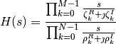
$H(s) = \frac{ \prod_{k=0}^{M-1}\frac{s}{\zeta_k^R + \jmath\zeta_k^I} }{ \prod_{k=0}^{N-1}\frac{s}{\rho_k^R + \jmath\rho_k^I} }$

where ζ ^R and ζ ^I are the real and imaginary parts of the k^th zero, while ρ ^R and ρ ^I are the real and imaginary parts of the k^th pole. If a root (a pole or zero) is real, the imaginary part is specified as zero. If a root is complex, its conjugate must also be present. If a root is zero, then the term associated with it is implemented as s, rather than (1 - s/r) (where r is the root). If ρ_k^R then the k^th pole is stable.

laplace_nd

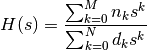
The laplace_nd filter implements the rational polynomial form of the Laplace transform filter. The general form is,

laplace_nd(operand[, n][, d][, epsilon])

Parameters:

operand (real) – signal to be filtered
n (real array) – numerator coefficients
d (real array) – denominator coefficients
epsilon (real) – tolerances

Return type:

real

where n is a vector of M real numbers containing the coefficients of the numerator and d is a vector of N real numbers containing the coefficients of the denominator. The transfer function is.

$H(s) = \frac{ \sum_{k=0}^{M}n_k s^k }{ \sum_{k=0}^{N}d_k s^k }$

laplace_zd

The laplace_zd filter is similar to the Laplace filters already described with laplace_zd accepting a zero/denominator polynomial form.

laplace_zd(operand[, zeta][, d][, epsilon])

Parameters:

operand (real) – signal to be filtered
zeta (real array) – zeros
d (real array) – denominator coefficients
epsilon (real) – tolerances

Return type:

real

laplace_np

The laplace_np filter is similar to the Laplace filters already described with laplace_np taking a numerator polynomial/pole form.

laplace_np(operand[, n][, rho][, epsilon])

Parameters:

operand (real) – signal to be filtered
n (real array) – numerator coefficients
rho (real array) – poles
epsilon (real) – tolerances

Return type:

real

Z Transform Filters

The z transform filters implement lumped linear discrete-time filters. Since they exist within analog processes, their inputs and outputs are continuous-time waveforms. Each filter function internally samples its input waveform x(t) to form a sequence x_n, it filters that sequence to produce an output sequence y_n, and then it passes that sequence through a zero-order hold to produce y(t). The input sampler is controlled by two parameters common to each of the filters, T and t₀. T is the sampling interval or time between samples and t₀ is the time of the first sample. The output zero-order hold is also controlled by two common parameters, T and τ. T is the total hold time for a sample and τ is the transition time, or the time the output takes to transition from one value to the next. During the transition, the output engages in a linear ramp between the old and new values so as to eliminate the discontinuous jump that would otherwise occur.

In addition to these three parameters, each z-domain filter takes three more arguments. The first is the input signal, x(t). The other two are vectors that describe the z-domain transfer function of the discrete-time filter. As with the Laplace filters, the transfer function can be described using either the coefficients or the roots of the numerator and denominator polynomials. The filter characteristics are static, meaning that any changes that occur during the course of the simulation in the values contained within these vectors are ignored; only their initial values are important.

The z transforms are written in terms of the variable z. The behavior of the internal discrete-time filter in the time domain can be found by convolving the inverse of the z transform with the input sequence, x_n. The composite behavior then includes the effect of the sampler and the zero-order hold. In frequency domain analyses, the transfer function of the digital filter is found by substituting z = exp(sT) where s = ⅉ2πf.

For quiescent operating point analyses, such as a DC analysis, the composite transfer characteristics are found by evaluating H(z) for z = 1.

Warning

The Cadence simulators do not implement the z transform filters in small signal analyses (AC, noise, etc.).

zi_zp

The zi_zp filter implements the zero-pole form of the z transform filter (zi is short for z inverse). The general form is

zi_zp(operand, [zeta, ][rho, ]T, tau, t0)

Parameters:

operand (real) – signal to be filtered
zeta (real array) – zeros
rho (real array) – poles
T (real) – period
tau (real) – transition time
t0 (real) – first sample time

Return type:

real

where zeta (ζ) is a vector of M pairs of real numbers. Each pair represents a zero, the first number in the pair is the real part of the zero frequency (in radians per second) and the second is the imaginary part. The zeros argument is optional. Similarly, rho (ρ) is the vector of N real pairs, one for each pole. The poles are given in the same manner as the zeros. The transfer function is,

$H(z) = \frac{ \prod_{k=0}^{M-1}\frac{z^{-1}}{\zeta_k^R + \jmath\zeta_k^I} }{ \prod_{k=0}^{N-1}\frac{z^{-1}}{\rho_k^R + \jmath\rho_k^I} }$

where ζ ^R and ζ ^I are the real and imaginary parts of the k^th zero, while ρ ^R and ρ ^I are the real and imaginary parts of the k^th pole. If a root (a pole or zero) is real, the imaginary part is specified as zero. If a root is complex, its conjugate must also be present. If a root is zero, then the term associated with it is implemented as s, rather than (1 - s/r) (where r is the root). If ρ_k^R then the k^th pole is stable.

zi_nd

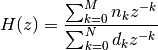
The zi_nd filter implements the rational polynomial form of the z transform filter. The general form is

zi_nd(operand, [n, ][d, ]T, tau, t0)

Parameters:

operand (real) – signal to be filtered
n (real array) – numerator coefficients
d (real array) – denominator coefficients
T (real) – period
tau (real) – transition time
t0 (real) – first sample time

Return type:

real

where n is a vector of M real numbers containing the coefficients of the numerator and d is a vector of N real numbers containing the coefficients of the denominator. The transfer function is.

$H(z) = \frac{ \sum_{k=0}^{M}n_k z^{-k} }{ \sum_{k=0}^{N}d_k z^{-k} }$

Example:

V(out) <+ zi_nd(V(in), {1}, {1}, 50u, 10u, 200u);

This example implements a simple sample and hold.

Example:

V(out) <+ zi_nd(V(in), {1}, {0, -1});

implements,

$H(z) = \frac{1}{1 - z^{-1}}$

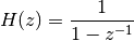
which is a backward-Euler discrete-time integrator.

zi_zd

The zi_zd filter is similar to the z transform filters already described with zi_zd accepting a zero/denominator polynomial form.

zi_zd(operand, [zeta, ][d, ]T, tau, t0)

Parameters:

operand (real) – signal to be filtered
zeta (real array) – zeros
d (real array) – denominator coefficients
T (real) – period
tau (real) – transition time
t0 (real) – first sample time

Return type:

real

zi_np

The zi_np filter is similar to the z transform filters already described with zi_np taking a numerator polynomial/pole form.

zi_np(operand, [n, ][rho, ]T, tau, t0)

Parameters:

operand (real) – signal to be filtered
n (real array) – numerator coefficients
rho (real array) – poles
T (real) – period
tau (real) – transition time
t0 (real) – first sample time

Return type:

real

Difference Equations and Z-Domain Filters

The z filters are used to implement the equivalent of discrete-time filters on continuous-time signals. Discrete-time filters are characterized as being either finite-impulse response (FIR) or infinite-impulse response (IIR). These filters are often defined in terms of difference equations. For example,

$y_n = \sum_{k=1}^{N} a_k y_{n-k} + \sum_{k=0}^{M} b_k x_{n-k}$

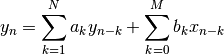
is a difference equation that describes an FIR filter if a_k = 0 for all k and an IIR filter otherwise. The transfer function of this transfer function is given by,

$H(z) = \frac{ \sum_{k=0}^{M}b_k z^{-k} }{ 1 - \sum_{k=1}^{N}a_k z^{-k} }$

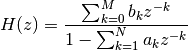
which can be implemented with a zi_nd filter if n_k = b_k for all k, d₁ = 1 and d_k = -a_k for k > 1.

Last Crossing

The last_crossing function returns a real value representing the time in seconds when its operand last crossed zero in a specified direction. The general form is

last_crossing(operand[, direction])

Parameters:

operand (integer) – signal
operand – direction

Return type:

real

If direction is +1 the function will observe only rising transitions through zero; if -1, falling transitions are observed; if 0, both rising and falling transitions are observed, and if any other value, no transitions are observed.

The last_crossing function does not control the time step to get accurate results; it uses interpolation to estimate the time of the last crossing. However, it can be used with the cross function for improved accuracy:

analog begin
   t = last_crossing(V(in) - vth, +1);
   @(cross(V(in) - vth, +1)) begin
      if (t0 > 0)
         $strobe("period = %rs (measured at %rs).", t - t0, $abstime);
      t0 = t;
   end
end

Note

$last_crossing is an analog operator and so must be placed outside the event block.

Limited Exponential

limexp(operand)

Parameters:: operand (real) – signal to be exponentiated
Return type:: real

The limexp function is an operator whose internal state contains information about the argument on previous iterations. It returns a real value that is the exponential of its single real argument, however, it internally limits the change of its output from iteration to iteration in order to reduce the risk of overflow and improve convergence. On any iteration where the change in the output of the limexp function is bounded, the simulator is prevented from terminating the iteration process. Thus, the simulator can only converge when the output of limexp equals the exponential of the input.

The apparent behavior of limexp is not distinguishable from exp, except using limexp to model semiconductor junctions generally results in dramatically improved convergence, though at the cost of extra memory being required.

Small-Signal Stimulus Functions

A small-signal analysis computes the steady-state response of a system that has been linearized about its operating point and is driven by one or more small sinusoids. The process of linearization eliminates the possibility of driving the circuit with conventional behavioral statements. The small-signal stimulus functions are provided to address this need; they operate after the linearization.

Note

Cadence simulators impose a restriction on the small-signal analysis functions that is not found in the Verilog-AMS standard. In Cadence’s simulators, the small-signal analysis functions must be alone in a contribution statement.

AC Stimulus (ac_stim)

SPICE-class simulators provide AC analysis, which is a small-signal analysis used for computing transfer functions. Verilog-A/MS provides the ac_stim function as a way of providing the stimulus for an AC analysis.

ac_stim([name], [mag], [phase]))

Parameters:

name (string) – active analysis name
mag (real) – magnitude
phase (real) – phase

Return type:

real

The AC stimulus function returns zero during large-signal analyses (such as DC and transient) as well as on all small-signal analyses using names that do not match name. The name of a small-signal analysis is implementation dependent, although the expected name (of the equivalent of a SPICE AC analysis) is "ac", which is the default value of name. When the name of the small-signal analysis matches name, the source becomes active and models a source with magnitude mag and phase phase. The default magnitude is one and the default phase is zero and is given in radians. Generally it is not necessary to give mag and phase unless there are multiple AC sources in your circuit.

Noise Stimulus (white_noise, flicker_noise, noise_table)

White noise processes are stochastic processes whose instantaneous value is completely uncorrelated with any previous or future values. This implies their spectral density does not depend on frequency. They are modeled using

white_noise( pwr, <name> )

white_noise(pwr[, name])

Parameters:

pwr (real) – output noise power
name (string) – noise type

Return type:

real

which generates white noise with a power density of pwr. The white_noise function can be used to model the thermal noise produced by a resistor as follows:

V(res) <+ r*I(res) + white_noise(4*`P_K*$temperature*r, "thermal");

The flicker_noise function models flicker noise. The general form is

flicker_noise(pwr[, exp][, name])

Parameters:

pwr (real) – output noise power
exp (real) – exponent
name (string) – noise type

Return type:

real

It produces noise with a power density of pwr at 1 Hz and varies in proportion to 1/f ^exp. The default value for exp is 1, which corresponds to pink noise (noise whose power is proportional to 1/f).

The noise_table function produces noise whose spectral density varies as a piecewise linear function of frequency. The general form is

noise_table(pwr[, name])

Parameters:

pwr (real array) – output noise power
name (string) – noise type

Return type:

real

where pwr is an array of real numbers organized as pairs: the first number in each pair is the frequency in Hertz and the second is the power. Noise pairs are specified in the order of ascending frequencies. The noise_table function performs piecewise linear interpolation to compute the power spectral density generated by the function at each frequency.

The amplitude of the signal output of the noise functions are all specified by their first argument in terms of a power density. It is important to understand that this is not a true power density that is specified in W/Hz. It cannot be because the noise function cannot know how its output is to be used. For example, the output may specify the noise voltage produced by a voltage source, but if the voltage source is not connected to a load then power produced by the source will be zero regardless of the noise amplitude. Instead, the amplitude of the noise is specified in a power-like way, meaning that if the units of the output signal for the noise function are U, then the units used to specify the noise density are U²/Hz. So, in this example, the noise power density is given in V²/Hz, which would be the true power if the source were driving a 1 Ω resistor. Similarly, if the output of the noise function were directly converted to a current, then the units of the power density argument would be A²/Hz, which is again the true power that would result if the current were passing through a 1 Ω resistor.

Each of the noise stimulus functions support an optional name argument, which acts as a label for the noise source. It is used when the simulator outputs a report that details the individual contribution made by each noise source to the total output noise. The contributions of noise sources with the same name from the same instance of a module are combined in the noise contribution summary.

File Operations

Verilog maintains a table of open files that may contain at most 32 files. Each file corresponds to one bit in a 32 bit integer that is referred to as a multichannel descriptor. The first bit, or channel 0, corresponds to the standard output. The first call to fopen opens channel 1, which corresponds to the second bit, etc. This non- traditional approach to files allows output to multiple files with a single statement.

File Open ($fopen)

The $fopen function takes a string argument that is interpreted as a file name and opens the corresponding file for writing. It returns an integer that contains the multichannel descriptor for the file. A 0 is returned if the file could not be opened for writing.

It also takes an optional mode parameter that takes one of three possible values: "w", "a" or "r". The "w" or write mode deletes the contents of the file if it exists before writing to it. The "a" or append mode appends the output to the existing contents of the specified file. In both cases, if the specified file does not exist, $fopen creates that file. The "r" mode opens a file for reading. An error is reported if the file does not exist.

For example:

integer f;

initial f = $fopen("results", "w");

always @(posedge clk) $fstrobe(f, "out = %b", out);

File Close ($fclose)

The $fclose task takes an integer argument that is interpreted as a multichannel descriptor for a file or files. It closes those files and makes the channels that were associated with the files available for reuse.

For example:

initial #1000 begin
   $fclose(f);
   $finish;
end