Introduction to Verilog-A
Verilog-A is the analog-only subset to Verilog-AMS. It is intended to allow users of SPICE class simulators create models for their simulations. Verilog-A models can be used in Verilog-AMS simulators, but in this case you would be be better served in most cases by using the full Verilog-AMS language. However, an initial step in learning the Verilog-AMS language is to learn Verilog-A.
Verilog-A, like Verilog, is a hardware description language. As such, it is quite different from programming languages. There are similarities of course, and knowing a programming language will help you to understand Verilog-A, but hardware description imposes much different goals and constraints on a language then general programming, and results in a much different language, one that might seem quite strange when unfamiliar. Unlike Verilog, which is a language intended to describe digital hardware, Verilog-A is intended to describe analog hardware. As such, Verilog-A is much different from Verilog, and may seem quite strange to anyone comfortable with Verilog.
Verilog-A is designed to describe models for SPICE-class simulators, or for the SPICE kernel in a Verilog-AMS simulator. SPICE simulators work by building up a system of nonlinear differential equations that describe the circuit that they are to simulate, and then solving that system of equations. Unlike in Verilog, the equations cannot be solved one at a time. They are a simultaneous system of equations that must all be solved all at once. Thus, one way in which SPICE differs from Verilog, in SPICE a solution point requires that all components be evaluated and all of the equations solved. This results in a SPICE representation of a circuit being much slower to simulate than a Verilog representation.
A module is a unit of Verilog code that is used to describe a component. In Verilog-A, as in Verilog, a circuit is described with a hierarchical composition of modules. In addition, both Verilog and Verilog-A allow built-in simulator primitives to be used in the circuit description. In Verilog, those built-in primitives generally describe gates. In Verilog-A, the built-in primitives describe common circuit components, such as resistors, capacitors, inductors, and semiconductor devices. A module that simply refers to other modules is often referred to as a structural model, or a netlist. Conversely, a module that uses equations to describe a component is referred to as a behavioral model. A module may contain both equations (behavior) and instantiations of other modules (structure). It also may contain neither, in which case it is referred to as an empty module.
SPICE uses Kirchhoff’s laws to formulate the circuit equations. In particular, it uses Kirchhoff’s potential and flow laws that are generalization of Kirchhoff’s voltage and current laws which extends these laws to voltage-like (potential) and current-like (flow) quantities. Kirchhoff’s potential law says that the sum of the potentials around any loop must be zero. Kirchhoff’s flow law says that the sum of flows into a node must be zero. SPICE combines the equations of the individual components with equations representing Kirchhoff’s laws to formulate the system of equations that it solves when simulating the circuit.
In Verilog-A, components are constructed using nodes and branches. A node is a point where the endpoints of branches may connect, and a branch is a single path between two nodes. To enforce Kirchhoff’s laws, the simulator places the following constraints on nodes and branches:
The potential is the same everywhere on a node
The flow onto the node must always sum to zero.
The potential on a branch is equal to the difference of potentials of the nodes to which it is connected.
The flow into one end of a branch is always equal to the flow out of the other end.
You can describe any arbitrary component with a collection of nodes and branches. That description consists of two things: the way that the nodes and branches are connected (their topology), and the way in which the potential and flow are related on each branch (the branch relations). Thus, to describe a component in Verilog-A you must: define the nodes and branches, and then specify the behavior of each branch. To see how this is done, consider this simple example of a linear two-terminal resistor:
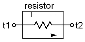
module resistor (t1, t2);
electrical t1, t2;
parameter real r=1;
branch (t1, t2) res;

analog V(res) <+ r*I(res);
endmodule
The first line defines the name of the component, in this case resistor, and the pins, which are nodes that the component shares with the rest of the circuit. Pins are also referred to as ports or terminals. In this case the pins are t1 and t2. The second line declares the pins as being electrical, meaning that the potential of each pin is a voltage and the flow into the pin is a current. Verilog-A defines the flow on the pin to be positive if the motion is into the component. The third line declares a parameter (r) for the component. Parameters are values that can be specified when you instantiate the resistor (when you place a resistor into your circuit). The value or r given in the parameter declaration is the default value of the parameter, it is the value used if no value is given during instantiation. Parameters are treated as constants within the module, meaning that the value of r cannot be changed from within the module. The fourth line declares a branch named res and indicates that it is connected between the t1 and t2 pins.
Important
The branch voltage V(res) equals V(t1) - V(t2), the difference in the voltages on the two terminals taken in the order given. Thus, the branch voltage is positive if the voltage on the first node listed in the declaration (t1) is greater than the voltage on the second node listed.
Important
The current of the branch is accessed using I(res). It is positive if the current flows from the first terminal specified when res was declared (t1) to the second terminal specified (t2).
At this point we have completed the topological portion of the description. The nodes and branches have been declared and arranged. We now know that there are two nodes, t1 and t2, that are shared with the rest of the circuit, and that there is a single branch, res, that connects t1 and t2.
The only thing left to do is to give the behavior of the branch; the branch relation. The branch has been connected to electrical nodes, so the branch itself must be electrical. Thus, a relationship between voltage and current is required. In Verilog-A all behavior is given in an analog process, which is denoted with the analog keyword. In this case, we only need one statement to define the behavior of the resistor, so it is sufficient to just give the analog keyword. If multiple statements are needed, then you would need to surround them with the begin and end keywords, as will be demonstrated shortly. The behavior of a branch is given using a contribution statement:
V(res) <+ r*I(res);
Use of the contribution operator (<+) makes this a contribution statement. It specifies an equation that must be satisfied by the simulator. It states that: the voltage on branch res must equal the current through that branch multiplied by r.
Using contribution statement is the only way to affect the value of a branch potential or flow (and indirectly the behavior of the greater circuit), and only branch potentials and flows may be the target of a contribution operator. Having said that, it is not always necessary to explicitly declare your branches. This resistor model could also have been given as:
module resistor (t1, t2);
electrical t1, t2;
parameter real r=1;

analog V(t1,t2) <+ r*I(t1,t2);
endmodule
In this case the resistor branch is created implicitly by combining t1 and t2 in the same access function. The voltage on t1 is greater than t2 if a positive value is contributed to the branch. The current on the branch is positive if it flows from t1 to t2.
The only way to affect the larger circuit is through branches. You can explicitly declare branches or create them on the fly. Whenever you do you must specify the terminals or end-points of the branch. Branches always have two terminals, but only one need be specified. If there is only one terminal specified, the one not specified is taken to be the second terminal and it is connected to ground. Voltage on the branch is positive if the voltage on the first terminal is greater than the voltage on the second. Current on the branch is positive if the current flows from the first terminal to the second.
Here is an example in which a branch is created by specifying only one terminal:
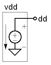
module vdd (dd);
electrical dd;
parameter real dc=2.5;

analog V(dd) <+ dc;
endmodule
If multiple contributions are made to the same branch, they accumulate. For example:
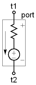
module port (t1, t2);
electrical t1, t2;
parameter real dc=0;
parameter real r=50;
branch (t1, t2) p;

analog begin
   V(p) <+ r*I(p);
   V(p) <+ dc;
end
endmodule
The behavior of the module is identical to the following module:
module port (t1, t2);
electrical t1, t2;
parameter real dc=0;
parameter real r=50;
branch (t1, t2) p;

analog V(p) <+ r*I(p) + dc;
endmodule
Whenever multiple contributions are made to a potential, they form a series combination. If multiple contributions are made to a flow, they combine in parallel. For example:
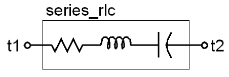
module series_rlc (t1, t2);
electrical t1, t2;
parameter real r=1;
parameter real l=1;
parameter real c=1 exclude 0;

analog begin
   V(t1,t2) <+ r*I(t1,t2);
   V(t1,t2) <+ l*ddt(I(t1,t2));
   V(t1,t2) <+ idt(I(t1,t2))/c;
end
endmodule
This module models a series combination of a resistor, a capacitor, and an inductor. It uses the idt and ddt operators to describe the capacitor and inductor. They respectively return the time integral or time derivative of their arguments. Similarly, here is the module for a parallel RLC:
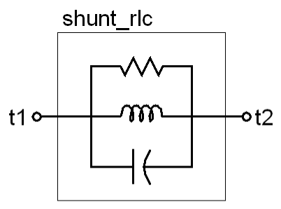
module shunt_rlc (t1, t2);
electrical t1, t2;
parameter real r=1 exclude 0;
parameter real l=1 exclude 0;
parameter real c=1;

analog begin
   I(t1,t2) <+ V(t1,t2)/r;
   I(t1,t2) <+ idt(V(t1,t2))/l;
   I(t1,t2) <+ c*ddt(V(t1,t2));
end
endmodule
Notice that in the serial RLC contributions were made to the voltage and in the parallel RLC contributions were made to the current. Constraining the contribution in this way can become awkward at times. For example, notice that in the series RLC it was necessary to use the integral form of the constitutive relationship for the capacitor. This form also divides by the capacitance, so the exclude clause was added to the declaration of c, which prevents the user from specifying a value of 0 for c. These restrictions are avoided if the branches are explicitly declared. For example, the shunt RLC can also described with:
module shunt_rlc (t1, t2);
electrical t1, t2;
parameter real r=1;
parameter real l=1;
parameter real c=1;
branch (t1, t2) res, ind, cap;

analog begin
   V(res) <+ r*I(res);
   V(ind) <+ l*ddt(I(ind));
   I(cap) <+ c*ddt(V(cap));
end
endmodule
In this case each component has its own branch, and the topology is defined by branch declarations rather than behavior of the contribution operator.
Rewriting the series RLC is a bit more complicated because it is also necessary to declare intermediate nodes:
module series_rlc (t1, t2);
electrical t1, t2, n1, n2;
parameter real r=1;
parameter real l=1;
parameter real c=1;
branch (t1, n1) res;
branch (n1, n2) ind;
branch (n2, t2) cap;

analog begin
   V(res) <+ r*I(res);
   V(ind) <+ l*ddt(I(ind));
   I(cap) <+ c*ddt(V(cap));
end
endmodule
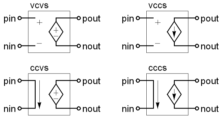
The following are the models of the common controlled sources:
// voltage controlled voltage source
module vcvs (pout, nout, pin, nin);
electrical pout, nout, pin, nin;
parameter real gain=1;

analog V(pout,nout) <+ gain*V(pin,nin);
endmodule
// voltage controlled current source
module ccvs (pout, nout, pin, nin);
electrical pout, nout, pin, nin;
parameter real gain=1;

analog I(pout,nout) <+ gain*V(pin,nin);
endmodule
// current controlled voltage source
module vccs (pout, nout, pin, nin);
electrical pout, nout, pin, nin;
parameter real gain=1;

analog V(pout,nout) <+ gain*I(pin,nin);
endmodule
// current controlled current source
module cccs (pout, nout, pin, nin);
electrical pout, nout, pin, nin;
parameter real gain=1;

analog I(pout,nout) <+ gain*I(pin,nin);
endmodule
There is one thing that is interesting about these models: they each use two branches but only describe the behavior of one of them. If a branch is employed but no behavior is specified for the branch, its behavior depends on how it is used. In these cases there are input and output branches, pin,nin and pout,nout. Behavior is given for pout,nout in the contribution statement. The behavior for pin,nin is not explicitly given in a contribution statement. In this case the default behavior is used. There are two possible default behaviors. If the potential of the branch is observed anywhere in the module, the flow is assumed to be 0, making it an ideal potential probe. If instead the flow of the branch were observed anywhere in the module, its potential is assumed to be 0, making it an ideal flow probe. It is illegal to observe both the potential and probe of a branch unless the behavior of the branch is explicitly specified with a contribution statement.
The four controlled sources also demonstrate one other feature of Verilog-A: the
single line comment. The double slash (//) introduces
a comment, anything that follows on that line is ignored. Verilog-A also
provides a multi line comment. Multi line comments begin with /* and end
with */. For example, you can hide a model from Verilog-A using:
/*
 * module vcvs (pout, nout, pin, nin);
 * electrical pout, nout, pin, nin;
 * parameter real gain=1;
 *
 * analog V(pout,nout) <+ gain*V(pin,nin);
 * endmodule
 */
It is not necessary to add the asterisk to the beginning of each line inside the comment, but it is a widely used convention to do so in order to emphasize the fact that those lines are being ignored by Verilog-A.